天蓝蓝年06月18日编写

Contents

实验3 线性系统的频率响应分析

clc
clear
close all
t=0:0.001:10;
w=[1,2,5,8,10,12,15,20,50,100];

num1=[100];
den1=[1 10 100];
        

绘制幅频特性

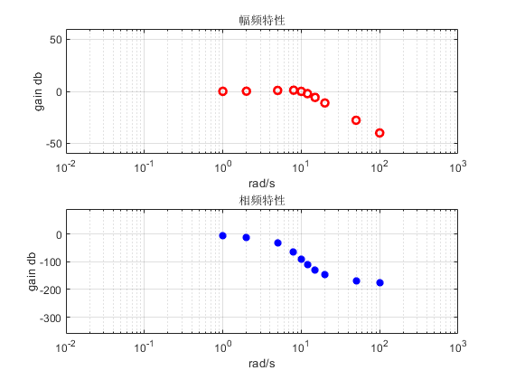
[magout,phase,w]=bode(num1,den1,w);
figure
subplot(2,1,1)
semilogx(w,20*log10(magout),'ro','Linewidth',2)
title('幅频特性');
xlim([0.01,1000])
ylim([-60,60])
xlabel('rad/s');
ylabel('gain db');
grid on;
subplot(2,1,2)
semilogx(w,phase,'b*','Linewidth',2)
title('相频特性');
xlim([0.01,1000])
ylim([-360,90])
xlabel('rad/s');
ylabel('gain db');
grid on;
% %% 绘制极坐标图
figure
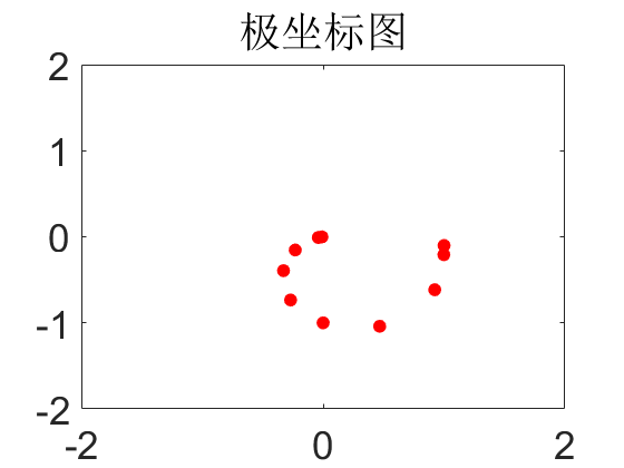
center=[0 0];%圆心坐标
for i=1:length(magout)
    x(i)=cos(phase(i)*pi/180).*magout(i)+center(1);
    y(i)=sin(phase(i)*pi/180).*magout(i)+center(2);
end
plot(x,y,'LineStyle','none','Marker','.','color','r','MarkerSize',30)
title('极坐标图')
% hold on
% for i=1:length(magout)
%     str=strcat('w=',num2str(w(i)),'rad/s');
%     text(x(i),y(i),str,'Color','k','FontSize',10);
% end
xlim([-2,2])
ylim([-2,2])
set(gca,'FontSize',26)

绘制时域特性

[magout,phase,w]=bode(num1,den1,w)
sys1 = tf(num1,den1)
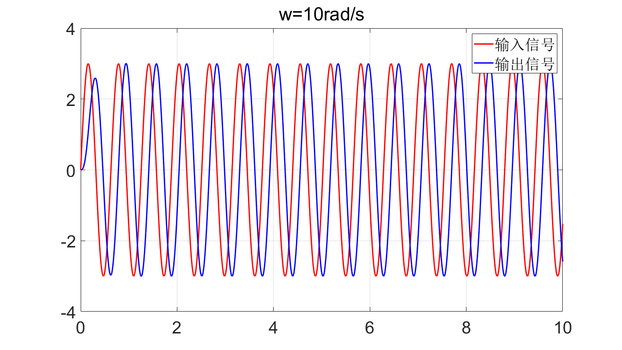
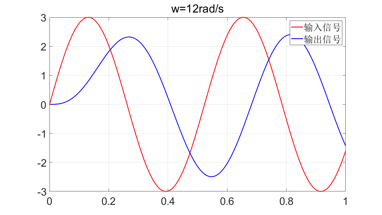
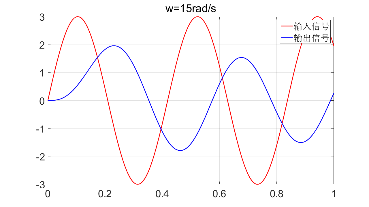
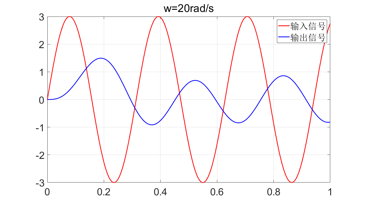
for i=1:length(w)
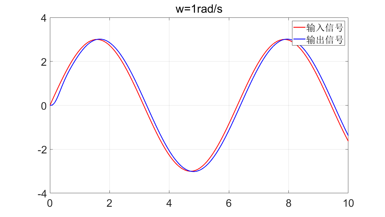
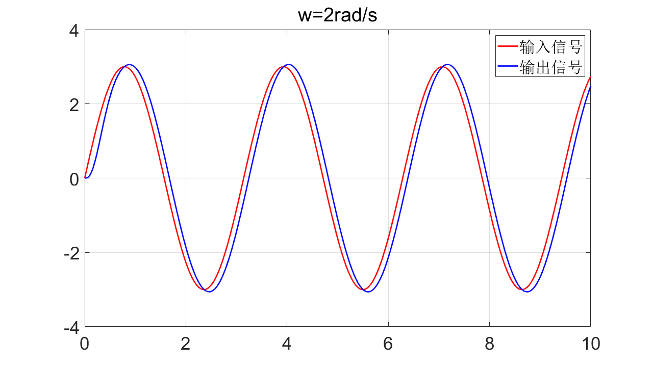
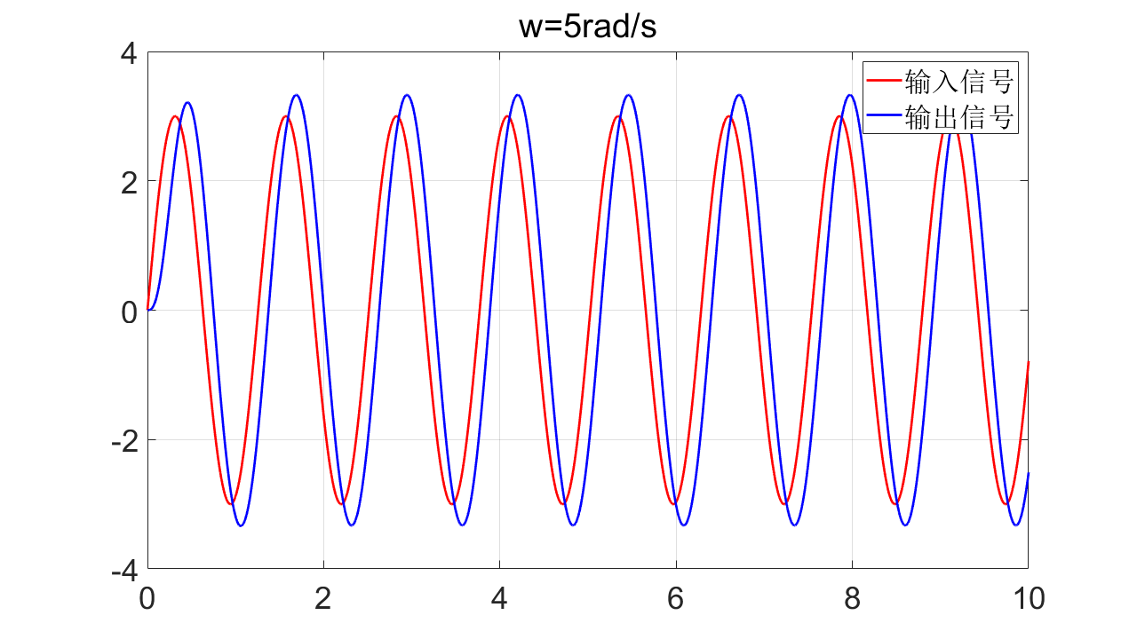
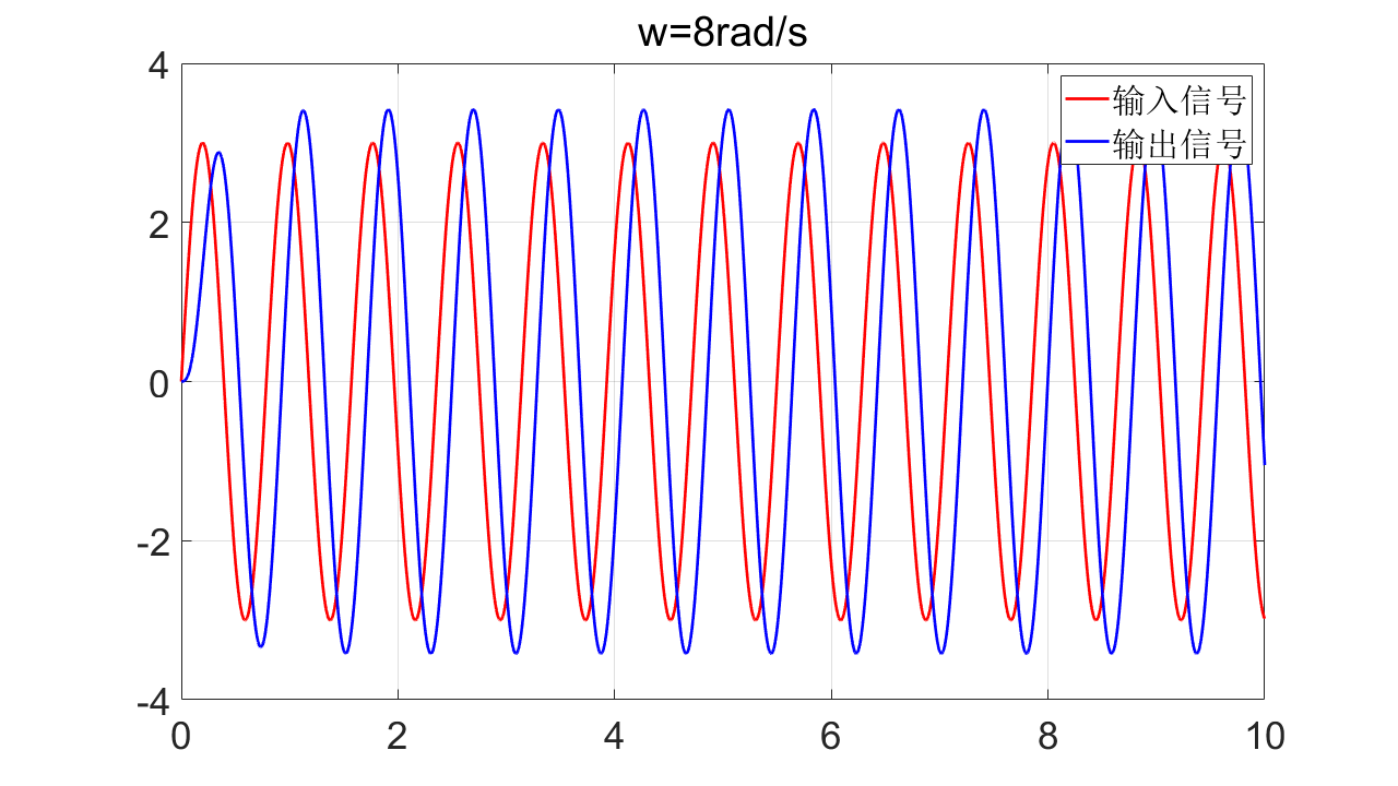
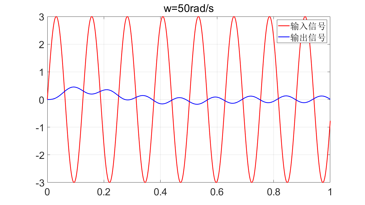
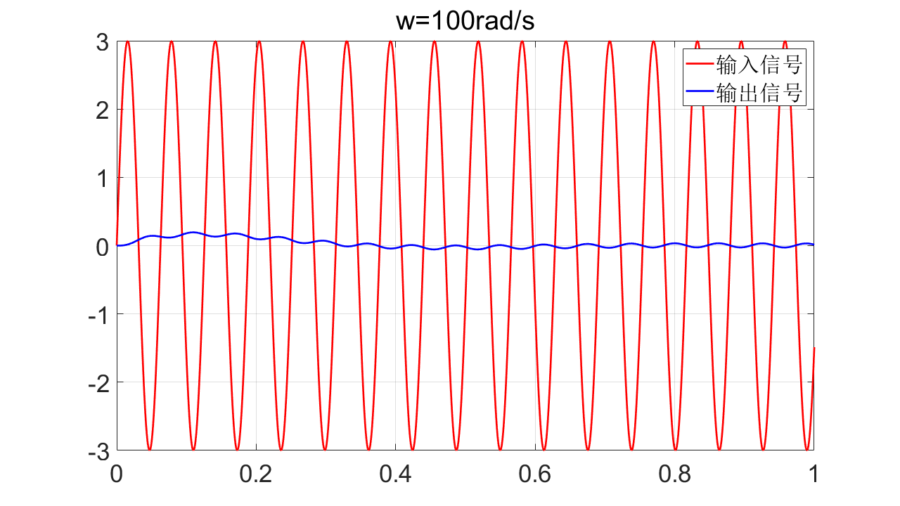
    yin=3*sin(w(i)*t);
    yout=lsim(sys1,yin,t);
    Yout(i,:)=yout;
    if i>5
        figure
        plot(t,yin,'r-',t,yout,'b-','Linewidth',2)
        legend('输入信号','输出信号')
        str=strcat('w=',num2str(w(i)),'rad/s');
        title(str)
        xlim([0,1])
        grid on
        set(gca,'FontSize',26)
        set(gcf,'unit','normalized','position',[0.05,0.05,0.5,0.5]);
    else
        figure
        plot(t,yin,'r-',t,yout,'b-','Linewidth',2)
        legend('输入信号','输出信号')
        grid on
        str=strcat('w=',num2str(w(i)),'rad/s');
        title(str)
        set(gca,'FontSize',26)
        set(gcf,'unit','normalized','position',[0.05,0.05,0.5,0.5]);
    end

end

magout =

    1.0050
    1.0198
    1.1094
    1.1399
    1.0000
    0.7824
    0.5121
    0.2774
    0.0408
    0.0100


phase =

   -5.7679
  -11.7683
  -33.6901
  -65.7723
  -90.0000
 -110.1363
 -129.8056
 -146.3099
 -168.2317
 -174.2321


w =

     1
     2
     5
     8
    10
    12
    15
    20
    50
   100


sys1 =
 
        100
  ----------------
  s^2 + 10 s + 100
 
Continuous-time transfer function.

Published with MATLAB® R2021b